

If you use TEA and LCA to judge the same cultivated meat waste route, you should expect different answers. That is not a modelling failure. It happens because TEA tests cost risk inside the plant, while LCA tests impact risk across the full life cycle.
For bioprocess engineers, cell culture scientists and cultivated meat R&D teams, the core point is simple: keep the same mass and energy balance, the same waste pathway, and the same basis of 1 kg edible product - then let each method do its own job.
Here’s the article in one pass:
- TEA asks: What does this waste route do to £/kg, CAPEX, OPEX and break-even?
- LCA asks: What does the same route do to GHG emissions, water use, land use, eutrophication and toxicity?
- Waste choices such as on-site treatment, outsourced disposal and media recovery can shift both models at once.
- In TEA, main sources of spread include media cost, recovery yield, utility system design, disposal charges, labour and policy assumptions.
- In LCA, main sources of spread include electricity mix, allocation rules, functional unit choice, transport distance and missing inventory data.
- A single assumption can swing LCA hard: the article cites 2.5 vs 13.5 kg CO₂-eq per kg product from a change in electricity mix alone.
- Media recovery can also move both models hard: the article cites 60–90% lower growth-media demand in circular recovery cases.
- So a route can look low-cost in TEA and still look high-impact in LCA, or the other way round.
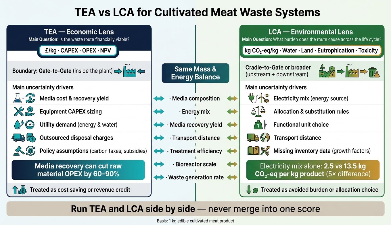
TEA vs LCA for Cultivated Meat Waste Systems: Key Differences at a Glance
The costs and environmental impacts of cultivated meat
sbb-itb-ffee270
Quick Comparison
| Point | TEA | LCA |
|---|---|---|
| Main question | Is the route financially viable? | What burden does the route cause across the life cycle? |
| Main output | £/kg, CAPEX, OPEX, NPV | kg CO₂-eq/kg, water, land, energy, eutrophication, toxicity |
| Typical boundary | Gate-to-gate | Cradle-to-gate or broader |
| Main uncertainty drivers | Price swings, scale-up, yield, utilities | Electricity mix, allocation, data gaps, transport |
| Waste recovery treatment | Cost saving or credit | Avoided-burden or allocation choice |
| Best use | Compare process options on cost | Compare process options on impact |
My takeaway: don’t blend TEA and LCA into one score. Run them side by side, report the assumptions plainly, and compare waste-route rankings only after you have matched the inventory, boundary and reporting basis.
TEA: How Economic Uncertainty Is Modelled for Cultivated Meat Waste Systems
In TEA, waste handling is treated first as an economic issue. Each choice - on-site treatment, outsourced disposal, or circular recovery - shows up as a cost or, in some cases, a credit. That makes the model useful for one practical reason: it shows exactly which assumptions are doing the heavy lifting. For waste systems, the main job is to identify which cost drivers matter most for each route.
Boundary, Data Inputs and Core Cost Drivers
TEA usually uses a facility-level, gate-to-gate boundary. In plain terms, it costs what happens inside the plant: CAPEX, OPEX, labour, utilities, maintenance, and storage. Upstream inputs are wrapped into purchase prices, while downstream effects are usually left out. That keeps the model manageable, but it also means impacts beyond the facility gate are not counted.
Within that boundary, the main inputs for waste-system TEA are CAPEX for treatment or recovery equipment, utility demand, labour, maintenance, and transport and storage charges for off-site handling. If the waste stream is recovered instead of discarded, that route can also generate a credit by displacing purchased inputs.
Because media is the dominant cost in cultivated meat TEA, recovery routes can shift waste-handling economics in a material way.
| TEA Uncertainty Source | Waste-System Input Affected | Economic Output Affected |
|---|---|---|
| CAPEX assumptions | Equipment sizing for on-site treatment | Annual cost; break-even conditions |
| Market price uncertainty | Cost of outsourced disposal vs byproduct recovery chemicals | Unit treatment burden; option comparison |
| Yield variability | Mass balance of spent media and nutrient recovery efficiency | Unit production cost; media cost savings |
| Utility demand | Energy and water use for sterilisation and aeration | Annual cost |
| Policy assumptions | Carbon taxes or renewable energy subsidies | Net present value; policy benefit |
These are the same inputs carried into the uncertainty analysis.
Sensitivity, Scenarios and Probabilistic TEA
TEA usually deals with uncertainty in three ways: sensitivity analysis, scenario analysis, and probabilistic methods such as Monte Carlo simulation. Sensitivity analysis changes one variable at a time, so you can see which inputs move the result most. Scenario analysis compares whole operating cases, such as batch versus continuous manufacturing. Probabilistic TEA changes several inputs at once and gives a range of likely outcomes instead of one point estimate.
It also helps to separate two different types of uncertainty. Model uncertainty refers to future values that are fixed in principle but still unknown, such as commercial-scale equipment costs or long-term outsourcing charges. Operational variability refers to process fluctuations, such as shifts in cell growth rate or yield during differentiation. Both affect waste-system outputs, but they are not the same thing and should be kept separate in the analysis.
Primary pilot or industrial data can reduce model uncertainty. This is particularly critical when navigating the challenges of scaling cultivated meat from pilot to industrial volumes. After that, sensitivity, scenario, and probabilistic analysis are used to test what is still uncertain.
The same waste scenario is handled differently in LCA, where the focus moves from cost to environmental impact.
LCA: How Environmental Uncertainty Is Modelled for the Same Waste System
LCA looks beyond the plant gate. It includes upstream burdens from electricity, fuels, chemicals, transport and consumables. That’s a key difference from narrower process assessments, and it starts with how the system boundary and inventory are defined.
Functional Unit, Life-Cycle Boundary and Inventory Needs
The first choice in any waste-system LCA is the functional unit: the basis used for comparison. That could be one kilogram of waste treated, or one kilogram of cultivated meat produced. The choice matters. Comparing results on a mass basis versus a nutrition-based basis such as protein content can change how the system compares with conventional meat, especially for water and land use [1].
After that, the inventory has to be built. For waste-system LCA, that usually means waste composition, treatment yields, emissions factors, electricity mix, transport distances and infrastructure linked to end-of-life treatment [1][2]. Sourcing these components through a cultivated meat B2B marketplace can help standardize inventory data. In practice, many of these inputs still come from proxy or literature data, which adds uncertainty. Primary supplier data can shift results in a big way when upstream land-use change differs.
Impact Categories, Monte Carlo and Model Choices
Waste-system LCA usually tracks:
- GHG emissions
- Energy demand
- Water use
- Land occupation
- Eutrophication
- Acidification
- Toxicity
Each impact category responds in its own way to modelling choices. So the same waste route can look one way in one study and quite different in another.
Electricity mix is one of the main drivers of climate-impact uncertainty. Research shows that cultivated meat produced with a conventional energy mix can have a carbon footprint of up to 13.5 kg CO₂-eq per kilogram of product, while a sustainable energy mix can reduce that to 2.5 kg CO₂-eq per kilogram - a fivefold difference from a single input assumption [1][4]. For eutrophication and toxicity, the main issue is often missing data. Growth factors and recombinant proteins are often left out of LCA inventories because primary data is still limited [1][4].
To deal with this, LCA practitioners use Monte Carlo simulation. In plain terms, they run the model many times while varying inputs such as yield, energy demand and transport distance. Instead of one point estimate, they get a probability distribution. That makes it easier to see which assumptions drive the broadest spread in outcomes.
Allocation and substitution choices add another layer. If a waste stream is valorised, the model has to decide how to assign credits for avoided inputs. Those credits can be large. Circular recovery systems have been shown to cut growth media requirements by 60–90% [3].
So uncertainty doesn’t sit in one place. It moves across impact categories depending on boundary choices, allocation rules and missing inventory data. That’s why the same waste route can rank differently across studies.
| LCA Uncertainty Source | Impact Categories Affected | Modelling Consequence |
|---|---|---|
| Functional Unit Choice | All categories | Shifts the comparison baseline; mass versus protein content alters results for water and land use [1] |
| Electricity Mix | GHG, energy demand | Up to fivefold variance in carbon footprint (2.5 vs 13.5 kg CO₂-eq per kg) [1][4] |
| Allocation Method | All categories | Determines whether environmental burden sits with the waste or the primary product [1] |
| Data Quality (growth factors excluded) | Toxicity, eutrophication, acidification | Excluding growth factors can understate impacts across these categories [1][4] |
The model is sensitive to boundary and allocation choices before any process data is entered. Two studies looking at the same waste route can reach different conclusions without either one being wrong, simply because they made different but defensible choices on boundary setting, allocation and substitution. That’s a big part of why TEA and LCA often diverge.
Where TEA and LCA Diverge and Why Results Often Conflict
TEA and LCA answer different questions. TEA asks whether a waste route works financially. LCA asks what that same route does across its environmental footprint. So it’s not unusual for one route to look good in TEA and less good in LCA.
The same waste pathway can rank differently because the two methods use different system boundaries, allocation rules, and data inputs. In practice, the split shows up most clearly in boundary, allocation, and data choice.
Boundary, Allocation and Data Divergence
TEA usually sets the boundary at the plant level. It focuses on what happens inside the process and what that means for cost, cash flow, and return. LCA extends the boundary upstream and downstream so it can include cultivated meat inputs sourcing, electricity mix, and waste emissions [1][2].
That difference matters straight away. If a waste stream is recovered or valorised, TEA will often treat it as a lower disposal cost or a revenue offset. LCA handles the same stream in a different way. It has to assign environmental burdens across co-products through allocation rules [1][3].
So a recovered material can improve process economics while still carrying a high environmental burden. From a TEA view, it may cut OPEX or add product value. From an LCA view, the same route may still look heavy once upstream inputs, energy demand, or emissions from treatment are counted.
How a Low-Cost Route Can Still Carry a Higher Environmental Burden
Waste handling makes this easy to see. A cheaper off-site disposal route can still perform worse in LCA if transport distances are longer, treatment uses more energy, or emissions are higher.
The reverse logic also holds. A waste route that lowers operating burden at the facility can still increase upstream emissions or transport impacts. So when TEA and LCA disagree, the problem is not accuracy. It comes from objective, boundary, and data choice.
Using TEA and LCA Together Without Mixing Their Outputs
TEA and LCA can rank the same waste route in different ways. That’s why they should run side by side, not be forced into one combined score. Keep the outputs separate, but make sure both models use the same inventory, the same functional unit, and the same system boundary.
A Shared Input Set for Both Models
Both models should start from one shared mass and energy balance: a single inventory covering waste generation rates, media composition, utility demand, treatment efficiency, transport distance, chemical consumption, and recovery yield [1][2]. The physical flows do not change between models; what changes is how each model reads those flows.
TEA uses that shared inventory to calculate cost metrics. LCA uses the same inventory to build the life cycle inventory and estimate impacts. If you can use primary industrial data, even better. This is often facilitated by bioprocess control software that tracks real-time production metrics. It tightens both models and makes any side-by-side comparison easier to defend.
That shared inventory is the hand-off point between the two methods. The table below shows how the same waste-system driver can mean one thing in TEA and something else in LCA.
| Waste-System Driver | TEA Effect | LCA Effect |
|---|---|---|
| Media composition | Primary cost driver (up to 99% of baseline cost) [4] | High impact via raw material origin |
| Energy mix | Utility cost fluctuations | Carbon footprint shifts with the energy mix |
| Media recovery yield | Reduces raw material OPEX by 60–90% [3] | Lowers upstream footprint via avoided production |
| Transport distance | Logistics and fuel costs | Transport-related emissions |
| Treatment efficiency | Cost of chemicals and energy for treatment | Avoided pollution and effluent quality |
| Bioreactor scale | Capital expenditure (CAPEX) | Energy intensity per kg of product |
| Waste generation rate | Disposal fees and loss of raw material value | Eutrophication and waste treatment emissions |
Reporting Rules for Defensible Decisions
For a fair comparison, report TEA and LCA for the same scenario, but do not merge them into a single score. Compare rankings under matched assumptions rather than relying on one point estimate. State the system boundary, any credited co-products, the energy mix, and the allocation method. Set the economic and environmental cut-offs before the analysis starts.
FAQs
Why do TEA and LCA give different answers?
TEA and LCA often point in different directions because they answer different questions and draw the line around the system in different places.
TEA looks at economic feasibility and production cost. LCA looks at environmental impacts across the product life cycle.
The results can also split because each method depends on its own assumptions and data sets. In cultivated meat, that uncertainty is often higher, simply because large-scale production data is still limited.
Which assumptions matter most in each model?
In both TEA and LCA for cultivated meat, the biggest assumptions usually sit around culture media: what goes into it and what it costs. That makes sense. Media can shape both production economics and environmental impacts more than almost anything else in the process.
For LCA, the main assumptions tend to centre on the energy mix, media raw materials, and circularity options such as recycling or waste valorisation. For TEA, the biggest drivers are cell yields, bioreactor efficiency, and production scale. Because commercial-scale data is still limited, many studies lean heavily on hypothetical inputs.
How can I compare waste routes fairly?
Use consistent system boundaries across all routes. That means covering the same core activities each time: cell growth, media processing, scaffold recovery, and wastewater treatment. If those boundaries shift from one route to another, the comparison starts to drift.
Data quality matters just as much. Use primary data from industrial-scale models wherever possible, not rough lab-based proxies that can skew the result.
Include the full life cycle of inputs and outputs. That should cover recycling options for media and recovery pathways for by-products such as ammonia and lactate.


